
지난 포스팅에서 K-Nearest Neighbor과는 다르게, Linear Classifier는 W값만으로 predict가 가능하다는 장점과, 더 정확한 정보를 얻을 수 있다는 것이 장점이었습니다. f(x, W) = W*x+b라는 식으로, (CIFAR-10 기준으로) 10가지의 카테고리당 점수를 알 수 있었습니다. 고양이, 자동차, 개구리, 사진아래에는 Weight값들을 사진으로 나타내어, Linear Classifier가 알아낸 카테고리의 특징을 알아볼 수 있습니다.

이 사진은, w값이 랜덤이기에 일어나는 상황이라고 하였죠. 자동차를 제외한 두 가지 카테고리의 점수는 정답을 거의 맞히지 못하는 상황입니다. 그리고, w값이 랜덤이라는 점에서부터, 도대체 w값을 어떻게 바꾸어 나가야 제대로 된 점수를 얻을 수 있을까?라는 질문을 던졌었죠? 바로 그 질문에 대해서 오늘 알아볼 시간입니다.
아! 들어가기 전에, 이 위의 내용 중 잘 모르는 내용이 있다면, 이전 포스팅으로 돌아가서 다시 한번 Linear classifier에 대한 이해를 하시고, 아래 내용을 따라와주세요! 최소한 Linear Classifier부분은 완벽하게 이해가 되어 있어야 합니다!
좋은 weight를 찾기 위해 우리가 해야할 일은
- 훈련 데이터의 점수에 대한 불만을 정량화하는 손실 함수를 정의합니다.
- 손실 함수를 최소화하는 파라미터를 효율적으로 찾는 방법을 생각해 보세요.
# Loss function (=손실 함수, 오차 함수)
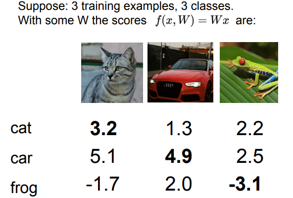
우선, 저번의 예제를 단순화시킨 곳으로 가봅시다. 고양이, 자동차, 개구리 세 가지의 카테고리밖에 없다고 가정하고, 그 각각의 점수만 나오는 것이죠. 예제를 보면, '고양이' 이미지는 자동차가 1등, 고양이가 2등, 개구리가 3등으로 나오고, '자동차' 이미지는 자동차가 1등, 개구리가 2등, 고양이가 3등으로 나오고, '개구리' 이미지는 자동차가 1등, 고양이가 2등, 개구리가 3등으로 나옵니다. 이렇게 된다면, '자동차' 이미지만이 정답을 맞혔고, 나머지 두 '고양이'와 '개구리'이미지는 정답을 맞히지 못한 것을 알 수 있습니다. 즉, 우리의 Linear Classifier가 썩 잘 작동하는 것은 아니라는 것이고, 우리는 이것을 고치고 싶습니다.
그래서 우리는 이러한 일에 대해 점수를 메기기로 했습니다. 과연 우리의 Linear Classifier가 얼마나 못하고 있는 걸까? 하는 것에 대한 점수죠. 이 점수를 우리는 Loss(오차)라고 합니다. 얼마나 정답에 오차가 있는가.. 하는 느낌이죠. 그리고, 그 Loss를 도출하는 함수가 바로 Loss function(오차함수)입니다.

위의 식을 한번 볼까요? 값은 이미지, 값은 그 이미지의 카테고리의 정답인, N개의 데이터셋을 가지고 있다고 해봅시다.

그렇다면, 전체 오차값인 L은 어떠한 오차 함수 Li에 우리의 Linear Classifier인 와 값을 집어넣은 값의 평균이라고 할 수 있습니다. 이러한 방식은, 다른 다양한 딥러닝 작업에 사용되는 오차값을 구하는 공식입니다. 그리고 이 안의 오차 함수가 무엇이 들어가느냐에 따라, 여러 가지 다른 오차값을 구할 수 있습니다.
이제부터 loss의 2가지 예를 살펴보겠습니다. Multicalss SVM(Support Vector Machine)을 이용한 Multiclass SVM loss(Hinge loss)와 Softmax function을 이용한 Cross entropy loss입니다. 먼저 Multiclass SVM loss를 살펴보겠습니다. (Multiclass SVM loss는 2개의 클래스를 다루는 SVM을 일반화 한 것입니다.)
# Multiclass SVM loss
그러면 여러가지 손실 함수 중 이미지 분류 문제에 적합한 손실함수인 SVM loss에 대해 살펴보겠습니다. SVM loss는 작동하는 방식이 굉장히 간단한 손실함수 중 하나입니다.


safty margin은 정답 클래스의 예측 점수가 다른 클래스의 예측 점수보다 최소 얼마나 더 커야하는지 정해줍니다. 정답 점수가 다른 점수에 비해 safety margin만큼 크지 않으면 loss가 생길 수 있습니다. safety margin이 1일 때, (정답 클래스의 예측 점수-오답 클래스의 예측 점수)가 1보다 크면 loss가 생긴다는 뜻입니다.
Loss를 구하는 방법은 정답 클래스 yi를 제외한 나머지 클래스 y의 합을 구하고 정답 클래스의 스코어와 오답 클래스의 스코어를 비교한다. 만약 정답 클래스의 점수와 오답 클래스의 점수의 격차가 safety margin이상으로 정답 클래스의 점수가 더 높으면 정답 클래스의 스코어가 다른 오답 클래스보다 훨씬 더 크다는 것을 의미합니다. 그렇게 되면 loss는 0이 됩니다. 이런식으로 정답이 아닌 클래스의 모든 값을 합치면 그 값이 바로 한 이미지의 최종 loss가 되는 겁니다. 그리고 전체 훈련 데이터 셋에서 그 loss들의 평균을 구하게 됩니다.
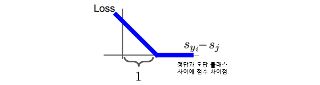
Multiclass SVM loss는 그래프의 모양이 경첩같이 생겨서 Hinge loss라고 부르기도 합니다. x좌표가 이미지의 정답의 예측점수이고, y축이 오차값이 된 그래프입니다. 정답인 클래스의 예측 점수가 오답인 클래스의 예측 점수보다 크면 Hinge loss는 작아집니다. 만약에 loss가 커지면 이미지를 잘 분류하지 못하고 loss가 0이면 이미지를 잘 분류해낸다는 뜻입니다.
Q. 음.. 잠시만요? 이러면 점수가 낮으면 좋은 건가요?
A. 네, 그렇습니다. 아까 말했다시피, 우리가 구하는 것은 오차값입니다. 얼마나 '틀려있나'의 정도를 나타내는 값이 오차값이라고 하였으므로, 이 점수가 낮다는 것은, 틀려있는 정도가 낮은 것이므로, 점수가 낮으면 낮을수록 더욱 정확하다고 할 수 있겠죠.
Q. 아니, 그런데 왜 그냥 현재 카테고리의 점수가 아니고, 현재 카테고리의 점수 + 1 값을 비교하고, 더해주는 거죠??
A. 만약 현재 카테고리의 점수 그 자체를 비교한다면, 2등의 점수와 1등의 점수가 굉장히 근사하다 하더라도, 오차값은 무조건 0, 즉 최고로 좋은 상태가 되어 있을 것입니다. 이런 상황은 우리가 그다지 반기는 상황이 아닙니다. 비록 정답은 맞혔다 하더라도, 굉장히 간당간당하게, 다르게 말하면 운 좋게 맞춘 꼴이 된 것이니깐요.. 그렇기 때문에, 더욱 확실히 정답을 맞히는 것을 목표로, +1을 더해주는 것입니다.
3개의 클래스(고양이/차/개구리)를 가지는 3개의 학습 데이터를 가정하고, W는 Linear Classifier를 따른다고 하고, Hinge loss를 직접 계산해본 결과입니다.
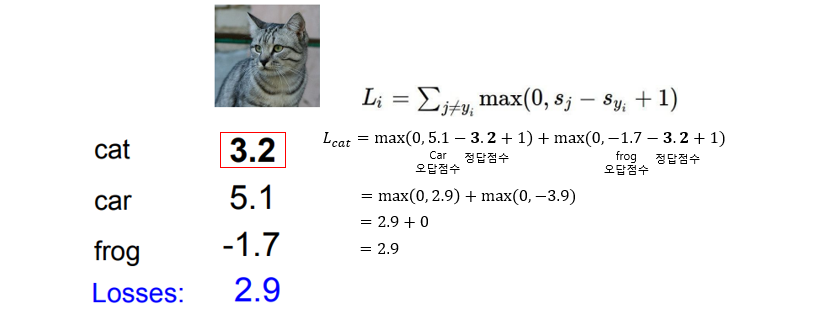
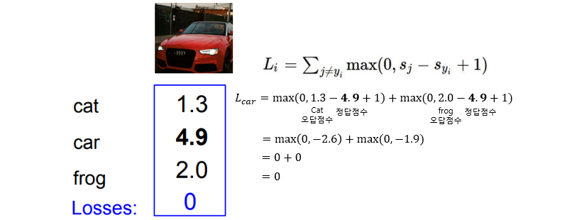
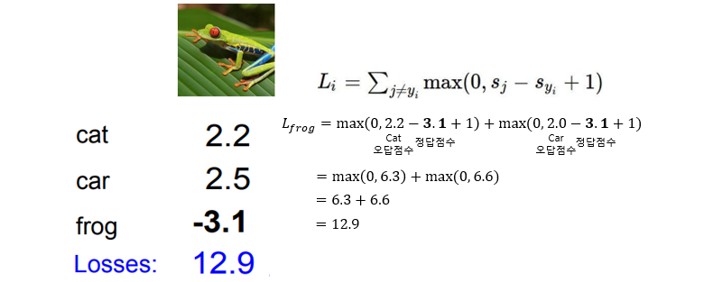

고양이의 Loss는 2.9, 자동차의 Loss는 0, 개구리의 Loss는 12.9의 결과로 볼 때, 자동차와 같이 정답을 맞춰야만 Loss는 0이 되는 것을 알 수 있습니다. 개구리 클래스를 보면 정답 클래스의 점수는 -3.1인데 오답 클래스인 cat과 car는 정답인 frog보다 크기때문에 Loss도 크게 계산된 것을 볼 수 있습니다. 따라서 각 클래스의 Loss의 평균은 5.27입니다. 이는 이미지를 잘 분류 못한다는 것입니다. Loss가 0에 가까울수록 이미지를 잘 분류하는 것입니다.
** 잘못된 레이블 스코어에서 제대로 된 레이블간 스코어 차에 일을 더한 값이 영보다 크면 그 값이 loss가 되고, 0보다 작으면 0이 레이블이 된다는 의미입니다.
Q. 자동차의 점수를 조금 바꾸면 Loss는 어떻게 되는가?
A. 변화가 없다. 자동차 클래스(정답 클래스)의 크기가 다른 오답 클래스의 점수보다 크기 때문에 Loss는 변함 없이 0이 된다. 그러나 만약 자동차의 점수가 2.0 이하(크게 변화)라면 Loss에 변화가 생긴다. (이해가 안 된다면 직접 수를 넣어 계산해 보자.)
Q. Loss의 최대값, 최소값은 무엇인가?
A. 정답 클래스의 점수가 클 때 Loss는 최소값인 0이 되고, 정답 클래스의 점수가 아주 큰 음수라면 Loss의 최대값은 ∞(무한대)가 된다.
Q. 일반적으로 가중치 W를 매우 작은 값으로 초기화한다. 그 때 모든 s는 0에 가깝게 된다. 이런 상황에서 Loss의 값은 무엇인가?
A. (클래스 수 - 1) (계산을 직접 해보면 알 수 있다.)
디버깅 전략(Sanity Check): W를 처음 학습할 때 Loss ≠ (클래스 수 -1)라면 버그가 걸렸다는 것을 알 수 있다.
Q. Loss 구하는 식이 정답을 포함한다면 Loss는 어떻게 될까?
A. Loss + 1이 된다. (직접 계산해 보자.)
Q. 합 대신에 평균을 사용하면 어떻게 될까?
A. Loss는 영향을 받지 않는다. Multiclass SVM loss function에서는 점수가 중요한 것이 아니라 점수의 상대적인 차이를 중요시 한다. 따라서 합 대신 평균을 사용하는 것은 점수의 차이를 단지 rescaling하는 것 뿐이다.

위의 식과 같이 제곱 항으로 바꾸면 결과가 달라집니다. 좋은 것과 나쁜 것 사이의 트레이드 오프를 비선형적인 방식으로 바꿔주는 것인데 그렇게 되면 손실함수의 계산 자체가 바뀌게 됩니다. 제곱 항을 고려하면 분류기가 만드는 다양한 Loss들 마다 상대적으로 패널티를 부여할 수 있습니다. Loss에 제곱을 한다면 이제 틀린 것들을 정말로 많이 틀린 것(나쁜 것)이 됩니다. 반면에 hinge loss는 "조금 잘못된 것"과 "많이 잘못된 것"을 크게 신경쓰지 않습니다. 둘 중 어떤 loss를 선택하느냐는 우리가 에러에 대해 얼마나 신경쓰고 있고, 그것을 어떻게 정량화 할 것인지에 달려있습니다.
# Multiclass SVM Loss : Example Code

def L_i_vectorized(x, y, w):
  scores = W.dot(x) # First calculate scores
  margins = np.maximum(0, scores - scores[y] + 1) # Then calculate the margins sj-sy+1
  margins[y] = 0 # only sum j is not y, so when j=y, set to zero
  loss_i = np.sum(margins) # sum across all j
  return loss_i
Loss가 0이 되게 하는 W를 찾았다면 그 W는 유일하게 하나만 존재하는 것일까? 다른 W도 존재합니다. 2W와 같이 스케일이 변해도 Loss가 0이 됩니다. W와 2W가 있다면, 정답 스코어와 정답이 아닌 스코어의 차이의 마진 또한 2배가 될 것입니다. 하지만 모든 마진이 이미 1보다 더 크다면 우리가 두배를 한다고 해도 여전히 1보다 클 것이고 Loss는 0입니다.
Loss=0이 되는 W를 고르는 것은 좋지 않을 수 있습니다. 그 이유는 training data에만 맞는 Loss function만 찾는 것이기 때문일 수 있습니다. 이 경우, test data를 넣었을 떄 이미지 분류기가 이해하지 못할 행동을 할 수도 있습니다.
# Softmax
Multinomial logistic regression, 즉, softmax는 딥러닝에서 자주 쓰입니다. multi-class SVM loss에서는 스코어 자체에 해석으로 고려하지 않고 단지 정답 클래스가 정답이 아닌 클래스들보다 더 높은 스코어를 내는 것을 원합니다. 하지만 Multinomial Logistic regression의 손실함수는 스코어 자체에 추가적인 의미를 부여합니다. softmax라고 불리는 함수를 쓰는데 스코어를 가지고 클래스 별 확률 분포를 계산합니다.


softmax함수는 스코어들을 가지고 스코어들에 지수를 취해 양수로 만들고 그 지수들의 합으로 다시 정규화 시킵니다. 그래서 softmax함수를 거치게 되면 확률분포를 얻을 수 있습니다. 그것이 바로 해당 클래스일 확률이 됩니다. 확률이기 때문에 0과 1사이의 값이 되고, 모든 확률들의 합은 1이 됩니다. 그래서 우리가 원하는 것은 정답 클래스에 해당하는 클래스의 확률이 1에 가깝게 계산되는 것입니다. 그렇게 되면 Loss는 "-log(정답클래스확률)"이 됩니다.
# Softmax 후 cross-entropy

확률적 해석에서는 따라서 정답 클래스의 음의 log likelihood를 최소화하고, 이는 Maximum Likelihood Estimation (MLE)를 수행하는 것으로 해석될 수 있습니다. 이 관점의 좋은 특징은 이제 전체 손실 함수의 정규화 항 R(W)를 가중치 행렬 W에 대한 Gaussian prior에서 나온 것으로 해석할 수도 있다는 것입니다. 여기서 MLE 대신 Maximum a posteriori (MAP) 추정을 수행하고 있다는 점입니다. 이러한 해석을 돕기 위해 이러한 유도의 전체적인 세부 사항은 이 강의의 범위를 벗어나기 때문에 언급합니다.
*** 정규항 R(W)은 다음 포스팅 regularization에서 다룹니다
*** Maximum Likelihood Estimation(MLE), Maximum a posteriori (MAP) : standford cs229에서 자세히 다룹니다

정보이론 관점에서 "정답" 분포 p와 추정된 분포 q 사이의 cross-entropy는 아래와 같이 정의 됩니다.

소프트맥스 분류기는 추정된 클래스 확률과 "정답" 분포 사이의 cross-entropy를 최소화합니다. 여기서 "정답" 분포는 모든 확률이 올바른 클래스에 할당된 분포입니다(정답 클래스에는 1, 정답이 아닌 클래스에는 0). 또한, cross-entropy는 entropy와 Kullback-Leibler divergence의 관계로 표현할 수 있으며 H(p,q)=H(p)+DkL(p∥q)로 쓸 수 있습니다. 델타 함수 p의 entropy는 0이므로 이는 두 분포 사이의 KL 발산을 최소화하는 것과 동일합니다. 다시 말해, cross-entropy목적은 예측된 분포가 모든 질량을 올바른 답변에 할당하도록 하려는 것입니다.
Q. 가능한 최소/최대 softmax loss Li는 무엇입니까?
A. softmax loss의 최솟값은 0이고, 최댓값은 무한대입니다.
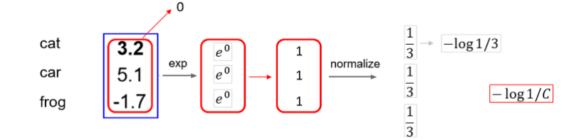
Q. 초기화 시 모든 sj는 대략 동일합니다. C클래스를 가정할 때 softmax loss Li는 얼마입니까?
A. 정답 클래스에 대한 log확률이기 때문에 log(1)=0이고 -log(1)=0이다. 그러므로 고양이를 완벽하게 분류했다면 loss는 0이다. loss가 0이 되려면, 실제 스코어는 극단적으로 높아야된다. 거의 무한대에 가깝게.. s가 모두 0근처에 모여있는 작은 수일 때, loss는 -log(1/c)가 되고, log(1/c)는 log(c)이다. loss식이 올바른지 확인하기 위해 sanity check를 위해 쓰일 수 있습니다.
만약 c=10, 10개의 클래스를 분류하고자 한다면 Li = Li=log(10) ~ 2.3
# Softmax : example code
f = np.array([123, 456, 789]) # example with 3 classes and each having large scores
p = np.exp(f) / np.sum(np.exp(f)) # Bad: Numeric problem, potential blowup

# instead: first shift the values of f so that the highest number is 0:
f -= np.max(f) # f becomes [-666, -333, 0]
p = np.exp(f) / np.sum(np.exp(f)) # safe to do, gives the correct answer
# Softmax vs SVM
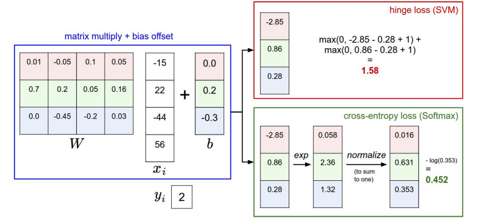
지금까지 배운 두 손실함수를 비교해보면 차이점은 얼마나 안좋은지를 측정하기 위한 스코어를 해석하는 방식이 조금 다르다는 것입니다. SVM에서는 정답 스코어와 정답이 아닌 스코어 간의 마진(margins)을 신경썼고, softmax분류기는 확률을 구해서 cross-entropy loss를 사용합니다. -log(정답클래스)에 신경을 썼습니다. SVM은 이를 클래스 점수로 해석하고 손실 함수는 올바른 클래스(파란색 클래스 2)가 다른 클래스 점수보다 약간 더 높은 점수를 갖도록 장려합니다. 대신 Softmax 분류기는 점수를 각 클래스에 대한 (정규화되지 않은) 로그 확률로 해석한 다음 올바른 클래스의 (정규화된) 로그 확률이 높아지도록 권장합니다(동일하게 해당 클래스의 음수는 낮음). 이 예의 최종 손실은 SVM의 경우 1.58이고 Softmax 분류기의 경우 1.04(기본 2 또는 기본 10이 아닌 자연 로그를 사용하는 1.04임)이지만 이 숫자는 비교할 수 없습니다. 이는 동일한 분류기 내에서 동일한 데이터로 계산된 손실과 관련해서만 의미가 있습니다.
Q. cross-entropy loss를 사용할 때 data값이 조금 변경되면 어떻게 될까?
A. loss는 확률 값으로 계산되기 때문에 조금만 데이터가 변경되어도 확률에 영향을 미쳐, loss가 변경하게 된다. hinge loss는 단순히 정답 레이블보다 1이상만 크면 영향을 미치지 않는다.
즉, cross-entropy loss(softmax)는 score값에 매우 민감한 것을 확인할 수 있다.
# reference
'Deep Learning > cs231n' 카테고리의 다른 글
| 쉽게 풀어쓴 cs231n 2강 Linear Classifier(2) (1) | 2023.11.23 |
|---|---|
| 쉽게 풀어쓴 cs231n 2강 Image Classification과 KNN(1) (3) | 2023.11.20 |